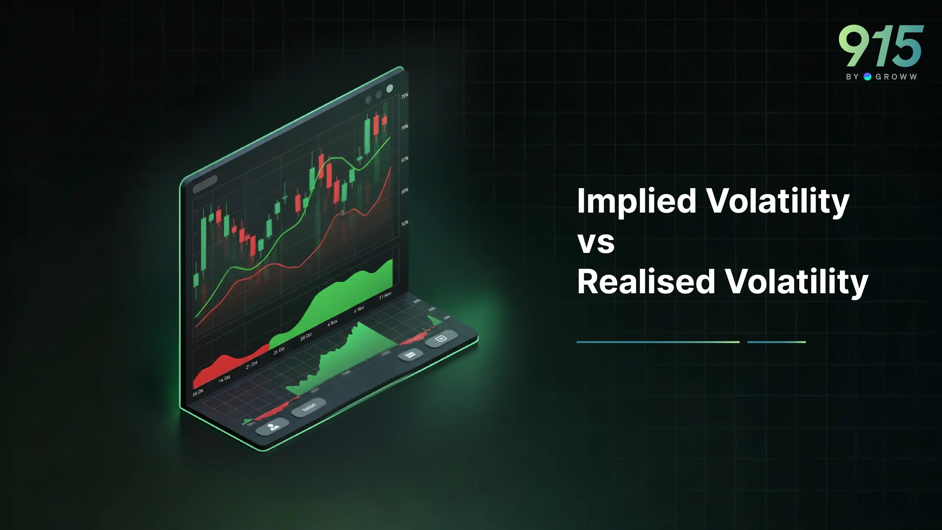
Implied Volatility vs Realised Volatility: Key Differences

What Is Realised Volatility?

Every asset moves. Some move fast, and some slow. The measure of the actual asset movement over a period is called Realised Volatility (RV). This movement has already occurred, so it is backwards-looking and computed directly from historical price data. 

For example, if Nifty has been moving a lot in the last 30 days, the RV will be high. On the other hand, if Nifty has been range-bound, the RV will be low.

Implied volatility, on the other hand, measures how much the market expects the underlying to move in the future. This is just an expectation and hence is forward-looking. The formula for Implied Volatility is derived from option prices. Usually, if the IV is high, then the options are expensive. If the IV is low, then the options are relatively cheap.

The Fundamental Relationship

Let's assume that the options are fairly priced. This means the RV equals IV. However, this is not always the case. Some reasons why RV will not equal IV are that uncertainty is always priced into options. And this gap drives much of the options' profitability.

Let's understand both scenarios now.

When IV > RV (Option Sellers Have Structural Edge)

If IV is higher than RV, it means the market expects higher volatility in the future. This results in options being traded at a higher premium. The extra premium is due to high volatility, and the premiums are inflated relative to actual movement. So some of the strategies that option writers can deploy during this time are:

• Short straddles/strangles
• Iron condors
• Calendars (sell front, buy back)
• Covered calls

When RV > IV (Option Buyers Have Edge)

On the other hand, if RV > IV, the expected volatility is low and the premiums are relatively cheap. Option buyers can take advantage of this, since options are priced cheaply relative to the underlying asset's movement. This leads to option buyers getting an explosive payoff. Some of the strategies that can be deployed are:

• Long straddles/strangles
• Directional call/put buying
• Event trades (if the move is bigger than the pricing)

Historical Behaviour Across Markets

It is interesting to note that, as per research across global markets (the US, India, Europe), IVs are generally higher than RVs over long horizons. This fact is known as Volatility Risk Premium. This is usually there to compensate overwriters for tail risk, gap risk, fat-tail events, and regime shifts.

This also gives rise to many systematic short-volatility strategies, which are known to work consistently for large hedge funds. 

Let's take a real-world example of how we can use IV and HV in trading. 

Suppose, for nifty options, the annualised IV is 22%. And the actual RV over the next 30 days was just 12%. This means that the Nifty moved less than expected. However, at the start, the options were overpriced. The option sellers would have been able to take advantage of this and made profits from theta as well as IV premium

On the other hand, if the expected IV is 14% and the actual RV is 25%, then the market moved more than it priced in. Option buyers would have made great profits from straddles and strangles. Option writers would have experienced large MTM swings and losses due to vega. 

Regime Shifts Are the Only Real Threat to Sellers

Volatility is mean-reverting. So even if volatility is high, option sellers can wait for it cool off and hence avoid losing big. However, there is a possibility of a regime where RV is unexpectedly above IV for a prolonged period. Some examples of RV regime spikes are the following:

• COVID crash
• 2008 GFC
• Brexit
• War announcements
• Currency crises
• Flash crashes

These are extreme events that lead to large losses for option writers. Vol sellers make money “slowly and steadily” until market shocks punish complacency. This is the right lens for viewing risk.

Conclusion

Many beginner option traders start with options with just directional bets in mind. They are essentially trading with just 1 aspect – delta. However, options are complex and encompass multiple option Greeks. Also, IV is very important for beginners to understand this before trading options. A lot of times, option buyers end up buying expensive options when the IV is high and selling options when the IV is low. Or they may ignore the volatility regime shifts. However, to be successful, traders should treat options like volatility products.