Calendar Spreads: Volatility, Theta & Term Structure Edge | 915

Option traders are of two types. Some use options just for trading the direction. If they expect the market to rise, they will buy a call option. And if they believe the market will go down, they will buy a put option. Some traders might create Option Strategies, such as a credit spread or a debit spread, but these strategies are also created with the direction in mind. However, the calendar spread is extremely different. In a Calendar spread, the aim is not to be right in the direction. It is purely a volatility-based trading strategy.

What Is a Calendar Spread?

Here is how to create a calendar spread:

• Selling a near-term option
• Buying a longer-dated option
• Both at the same strike price

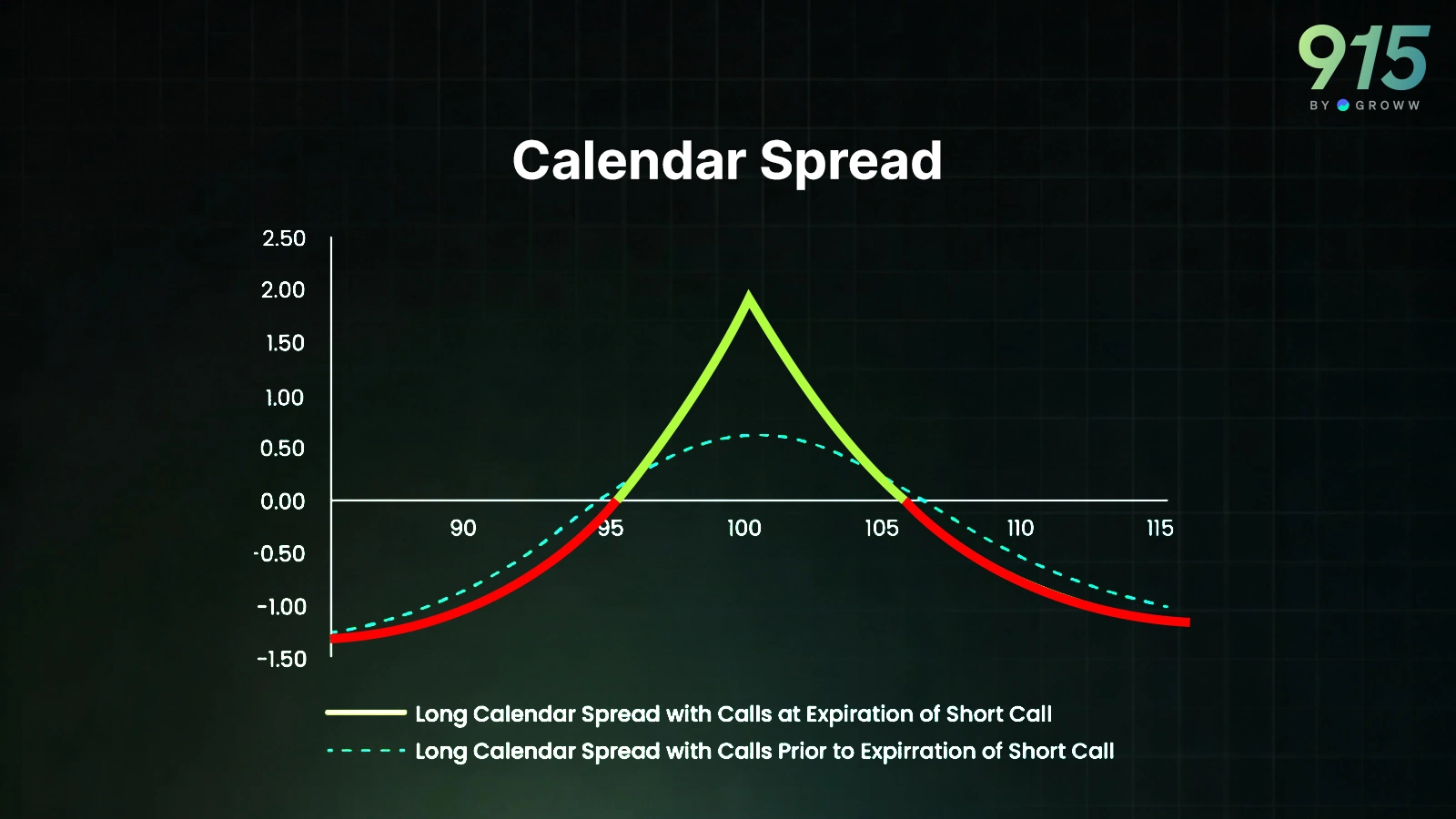
For example, let us assume the underlying stock is trading at ₹100. The strike price that we will be taking is ATM (100). In that case that trader will sell one near-month call and buy one next-month call.

The net cost of the spread is ₹3. This is the debit spread. This also shows the maximum theoretical risk in this strategy.

Let us do some scenario analysis now. Let us assume that after one week, the implied volatility has not changed. 

Case 1: If the price stays the same at ₹100, the breakup would be:

Case 2: If the price moves to ₹105, the breakup would be:

Case 3: If the price moves to ₹95, the breakup would be:

Here is the summary:

It is important to note that in a calendar spread, the near-expiry option is usually shorted and the far-expiry option is bought. This creates an interesting exposure profile:

• Net long Vega (sensitive to volatility increases)
• Net short Theta initially (benefits from faster decay in the short leg)
• Limited directional bias near the strike

This is why calendar spreads are often described as structured volatility trades.

Why Calendar Spreads Are Primarily a Volatility View

To understand this, think about what you are actually betting on.

Let us again see how the calendar spread is being formed. We are shorting near-term expiry options. And we are buying long-term expiry options. Short-term expiry options have higher theta decay and lose premium rapidly as the expiry approaches. On the other hand, the long-term expiry options have lower decay and greater sensitivity to volatility. So, the trade benefits when:

1. Near-term implied volatility stays stable or drops slightly.
2. Back-month implied volatility remains firm or rises.
3. Price stays near the strike into the front expiry.
4. Time passes, and the short option decays faster than the long option.

In essence, the calendar spreads exploit differences in implied volatility across expiries. This is also known as the volatility term structure. If short-dated volatility is currently higher than longer-dated volatility, you can sell the expensive short-term premium and buy the relatively cheaper longer-term volatility. The trader is now expecting volatility to normalise and revert to the mean. Once this is achieved, the spread is in the profit. 

The calendar spreads are best initiated when the price remains near the strike of the spread at the front expiry. If the price moves too far away, then the short leg may decay, but the long leg may lose extrinsic value. This may lead to the spread being flat or even losing a small amount of value. Hence, the traders usually place calendar spreads when the underlying is near a consolidation zone.

Sometimes, the spread is made when the trader is anticipating volatility expansion in later expiries.

Here are the thumb rules for when to trade the calendar spread:

• Front-month volatility is temporarily inflated.
• The market is expected to consolidate in the short term.
• Back-month volatility is underpriced relative to future uncertainty.
• Term structure is steep or distorted.

On the other hand, it is best to avoid the calendar spreads when:

• Price makes a large directional move immediately.
• Implied volatility collapses across all expiries.
• Term structure shifts unfavourably.
• Short volatility exposure in the front month expands sharply.

Conclusion

A calendar spread is one of the cleanest ways to express a relative volatility view. This option strategy allows traders to sell near-term options and buy far-term options. Usually, this is done on an ATM strike, which minimises the directional exposure. This is a pure bet on volatility, not on price. Strategy works well when the trader expects volatility to increase in the future.